Binary Segmentation: Cloud Detection with U-Net

The biggest challenge while working with remote sensing images is dealing with Clouds. If there are clouds all over the images you are trying to work with, well, you can’t really see anything through the clouds, right? So, it is important to know where clouds are and to filter those images that are useless.

A lot of cloud masking algorithms have been developed in the past years in order to detect clouds. For example, this paper reviews the existing Cloud detection methodologies.

An accurate cloud detection on remote sensing images is essential in projects such as land-use classification, crop yield prediction, crop monitoring, etc.
Photo by Hakan Yalcin on Unsplash

Computer Vision Task: Semantic Segmentation

In this article, we will use a semantic segmentation model called U-Net to detect the clouds on the satellite images.

So first, what is Semantic Segmentation?

You are probably familiar with classification which consists of attributing a class — or multiple classes — to objects. For example, we can classify an image as being a picture of a dog or a picture of a unicorn. Another way of classifying is to do classification and localization, also called object detection. In this case, we precise where the dog or unicorn is in the image using a bounding box around the object. Similarly, semantic segmentation attributes a class/several classes to each pixel of an image. It is a pixel-wise detection and classification. So, when trying to classify dog vs unicorn, instead of saying “this image is an image of a dog and the dog is on the right side of the image”, we say: “this pixel belongs to a dog”, and then, we have all pixels belonging to the dog object.

Here is a visual example that shows all the different types of computer vision tasks:

Now that we know what semantic segmentation is, let’s focus on our example of the day: Binary Semantic Segmentation of clouds. The main goal here is to find the pixels that belong to clouds and classify them as “cloud” while classifying the rest as “non-cloud”, hereby why we use binary semantic segmentation: we only have two classes.

Question we are trying to answer: Does this pixel belongs to a cloud or not?

38-Cloud: A Cloud Segmentation Dataset

In this tutorial, we will use the Kaggle 38-Cloud: Cloud Segmentation in Satellite Images dataset. This dataset gathers Landsat satellite images with visible clouds and their corresponding masks (ground truth):

• The images have 4 channels: Red, Green, Blue, and NIR (Near Infrared):

• The mask images are manually extracted pixel-level ground truths (0 = background and 255 = cloud)

Setting up the dataset in Hub

The data preparation step, including the part that sends the final dataset to the Hub storage, can take quite some time, and so I would advise using the final dataset accessible at the path: hub://margauxmforsythe/38-cloud-segmentation.

Structure of the dataset

Let’s take a look at how the dataset is organized:

So we can see that the different bands (R, G, B, NIR) are saved in separated subfolders: train_blue, train_green, train_red, train_nir.

We can start by visualizing some of the images in the dataset:

dataset_path = "./data/38cloud-cloud-segmentation-in-satellite-images/38-Cloud_training"

def read_image(path):
 img = np.array(Image.open(path))
 return img

def read_image_and_imshow(path):
 img = read_image(path)
 plt.imshow(img, cmap=’gray’) 
 plt.show()

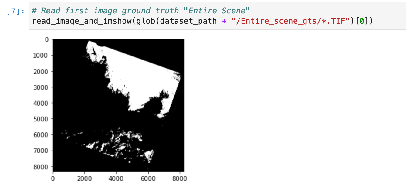
The dataset has 8 entire scene images. Patches are used for training because the entire scene images are too big, so, instead, 8401 patches of size 384x384 were generated from the original 8 entire scene images. Here is the first entire scene image in the dataset:

If we look at the first three ground truth (gt) patch images, we see that some patches are empty:

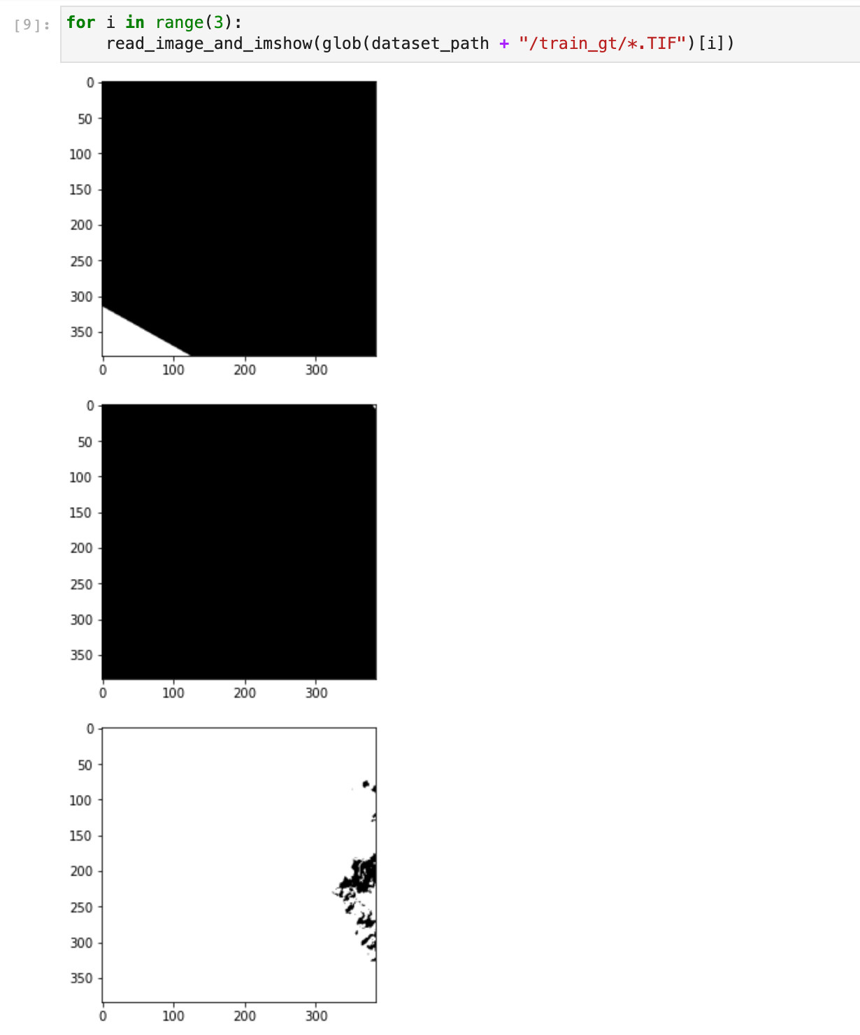
The second patch is empty, meaning the corresponding patch image has no cloud. We, therefore, used the CSV file training_patches_38-cloud_nonempty.csv to only have non-empty images. There are 5155 patches with clouds:

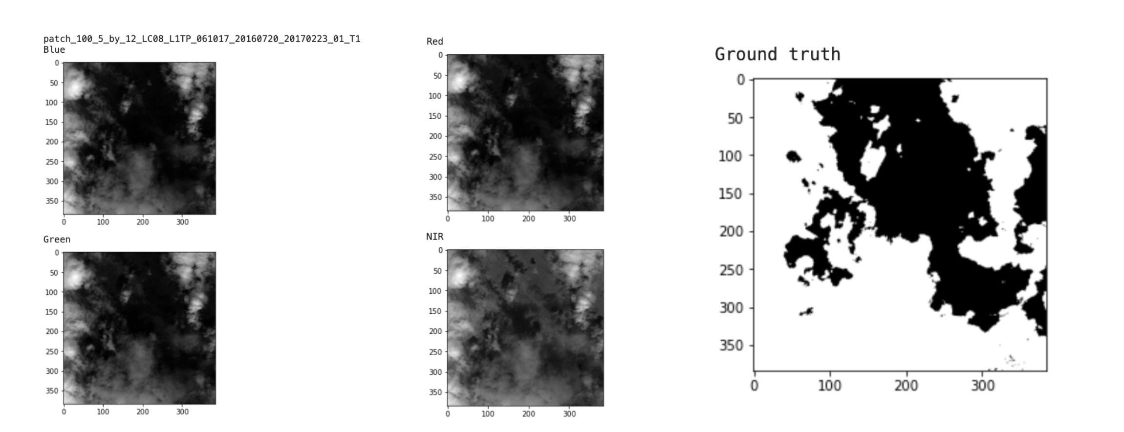
Now we want to take a look at each channel: Red, Blue, Green, NIR and the ground truth image:

list_training_files = list(training_files.name)

for image_name in list_training_files:
    print(image_name)
    print("Blue")
    read_image_and_imshow(f"{dataset_path}/train_blue/blue_{image_name}.TIF")  
    print("Green")
    read_image_and_imshow(f"{dataset_path}/train_green/green_{image_name}.TIF")
    print("Red")
    read_image_and_imshow(f"{dataset_path}/train_red/red_{image_name}.TIF")      
    print("NIR")
    read_image_and_imshow(f"{dataset_path}/train_nir/nir_{image_name}.TIF")    
    print("Ground truth")
    read_image_and_imshow(f"{dataset_path}/train_gt/gt_{image_name}.TIF")        
    break

We were able to visualize the different bands of this image, but remember that the bands are all saved in separated subfolders: train_blue, train_green, train_red, train_nir. For our training purposes, we want to combine all bands together.

Combine all bands together and send np arrays to Hub

In order to combine the bands of the image into one NumPy array, we first read the image using the path provided in the CSV file. Then, since images are 2D arrays (384, 384) and we need 3D arrays (384, 384, 1) to stack all the bands together, we use the NumPy function expand_dims to add a dimension to all the images. And finally, we use the NumPy concatenate function to combine the red, blue, green, and nir channels into one NumPy array of shape (384, 384, 4):

def combine_bands(dataset_path, image_path):
   path_red = f"{dataset_path}/train_red/red_{image_name}.TIF"
   path_green = f"{dataset_path}/train_green/green_{image_name}.TIF"
   path_blue = f"{dataset_path}/train_blue/blue_{image_name}.TIF"
   path_nir = f"{dataset_path}/train_nir/nir_{image_name}.TIF"
   path_gt = f"{dataset_path}/train_gt/gt_{image_name}.TIF"

   # Read images
   fnames = [path_red, path_green, path_blue, path_nir, path_gt]
   images = [read_image(fname) for fname in fnames]

   # Expand dimensions
   expanded_images = [np.expand_dims(img, axis=2) for img in images]

   # Combine red, blue, green and nir
   img_combined = np.concatenate(expanded_images[:4], axis=2)
   gt = expanded_images[-1]
   return img_combined, gt

If we test this function on the first image in the list:

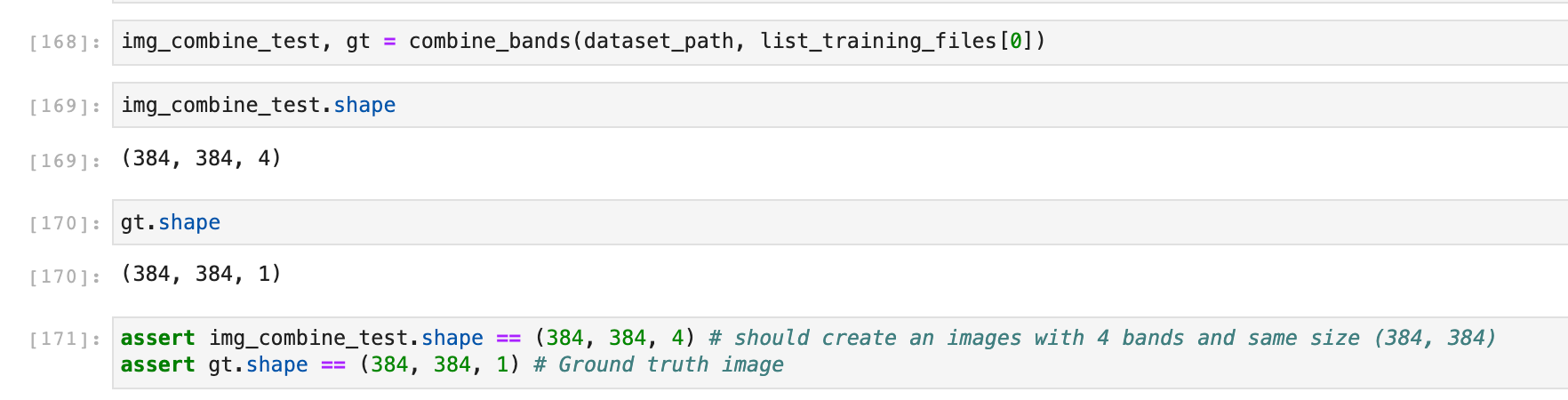
Now we can combine the bands of all the images in the list:

list_all_combined_images = []
list_all_masks = []

# Loop through all the image paths in the taining csv file
for image_name in tqdm(list_training_files):
    img, mask = combine_bands(dataset_path, image_name)
    list_all_combined_images.append(img)
    list_all_masks.append(mask)

# Convert lists to numpy arrays 
list_all_combined_images_np = np.array(list_all_combined_images)
list_all_masks_np = np.array(list_all_masks)

# Let's check if we have the right shapes
print(list_all_combined_images_np.shape) # (5155, 384, 384, 4)
print(list_all_masks_np.shape) # (5155, 384, 384, 1)

The output shapes are correct: we have 5155 images of shape (384, 384) with 4 bands each and their corresponding masks that only have one band which is the ground truth.

Now, we can send the arrays to the Hub. First, we need to login:

!activeloop login -u username -p password

Then, we chose the name of the Hub Dataset:

hub_cloud_path = "hub://margauxmforsythe/38-cloud-segmentation"

and populate it:

# This will take some time -- Go get a coffee :)
with hub.empty(hub_cloud_path) as ds:
    # Create the tensors 
    ds.create_tensor('images')
    ds.create_tensor('masks')

    # Add arbitrary metadata - Optional
    ds.info.update(description = 'Cloud segmentation dataset')
    ds.images.info.update(camera_type = 'SLR')

    # Iterate through the images and their corresponding embeddings,
    # and append them to hub dataset
    for i in tqdm(range(len(list_all_combined_images_np))):
        # Append to Hub Dataset
        ds.images.append(list_all_combined_images_np[i])  
        ds.masks.append(list_all_masks_np[i]) 

Done! Our cloud segmentation dataset is now saved in the Hub format and is accessible using the path “hub://margauxmforsythe/38-cloud-segmentation" and can be used from anywhere ☀️

The Notebook to prepare the data and send it to Hub can be found here (NB: this notebook was originally run locally with Jupyter).

Training in the Rain 🎵

“The way I see it, if you want the rainbow, you got to put up with the rain.” — Dolly Parton

Model: U-Net

We will use the semantic segmentation model architecture called U-Net. U-Net is a convolutional neural network (CNN) that was originally developed for biomedical image segmentation.

Loading data & splitting the dataset for training

First of all, we need to load the dataset from Hub:

# Load the data
print("Load data...")
ds = hub.dataset("hub://margauxmforsythe/38-cloud-segmentation")

Using the Connecting Hub Datasets to ML Frameworks feature, we can convert the dataset ds to Tensorflow format and perform the correct mapping and normalization:

# we choose to only use 100 images for training because of GPU limit capacity in Google Colab
image_count = 100
ds_tf = ds[:image_count].tensorflow()

def to_model_fit(item):
  x = item['images']
  # Normalize
  x = x / tf.reduce_max(x)
  y = item['masks'] / 255
  return (x, y)

ds_tf = ds_tf.map(lambda x: to_model_fit(x))

Visual sanity check:

for img, label in ds_tf:
  print(img.shape)
  print(label.shape)
  print(np.unique(label))
  plt.imshow(img[:,:,0])
  plt.show()
  plt.imshow(label[:,:,0], cmap="gray")
  plt.show()
  break

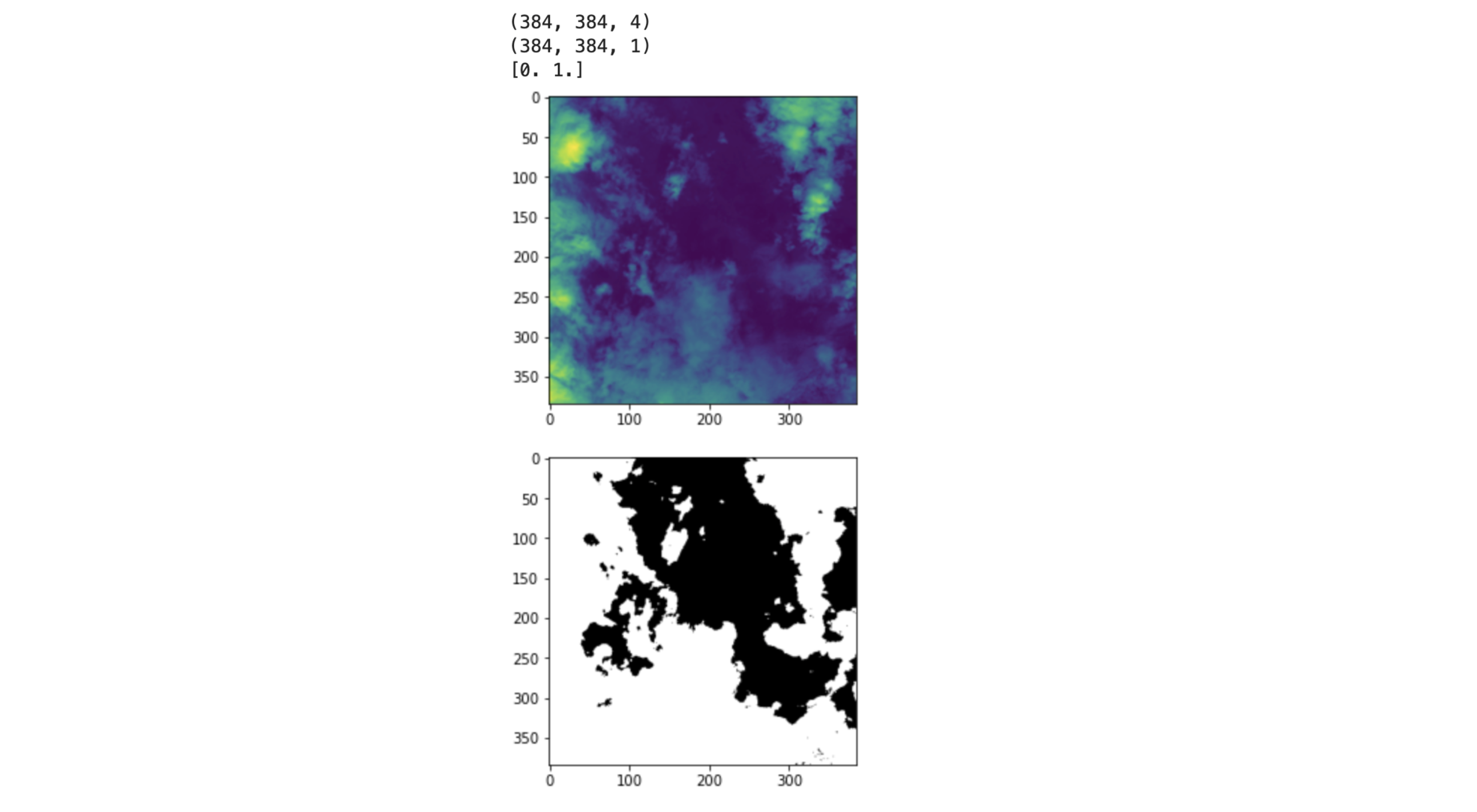
The image looks good, we have the image’s shape = (384, 384, 4) which is the correct shape since we have 4 bands. The shape of the mask is also correct (384, 384,1) since we have 1 band for the ground truth. And then finally, np.unique(label) returns [0,1] which is what we expected because we have two classes: cloud/non-cloud(background).

Now, let’s split the dataset:

train_size = int(0.8 * image_count)
val_size = int(0.1 * image_count)
test_size = int(0.1 * image_count)
batch_size = 6

ds_tf = ds_tf.shuffle(image_count)
test_ds = ds_tf.take(test_size)
train_ds = ds_tf.skip(test_size)
val_ds = train_ds.take(val_size)
train_ds = train_ds.skip(val_size)

print(f"{train_size} training images, {val_size} validation images and {test_size} test images. Batch size of {batch_size}")

train_ds = train_ds.shuffle(train_size)
train_ds = train_ds.batch(batch_size)

val_ds = val_ds.shuffle(val_size)
val_ds = val_ds.batch(batch_size)

test_ds = test_ds.batch(1)

=> 80 training images, 10 validation images, and 10 test images. Batch size of 6

Training hyperparameters and metrics

We have our train, validation, and test sets. We can now set up the hyperparameters and metrics for the training:

model = unet(input_shape = (384,384,4))

# Compile the model and use some good metrics for segmentation
model.compile(optimizer=tf.keras.optimizers.Adam(1e-4),
              loss='binary_crossentropy',
              metrics=['accuracy',
              tf.keras.metrics.Recall(name="recall"),
              tf.keras.metrics.Precision(name="precision"),
              tf.keras.metrics.MeanIoU(num_classes=2, name='iou')])

We use the binary cross-entropy loss because we are doing binary segmentation. Then we choose to use recall, precision, accuracy and iou as metrics.

We also define a callback to save the checkpoint when the iou score for the validation set is improving:

from tf.keras.callbacks import ModelCheckpoint

checkpoint_callback = ModelCheckpoint('./checkpoints/weights.epoch-{epoch:02d}-val-iou-{val_iou:.4f}.hdf5',
    monitor='val_iou',
    mode='max', 
    verbose=1,
    save_best_only=True,
    save_weights_only=True)

Training!

We are ready to start the training:

model.fit(train_ds, 
          validation_data=val_ds, 
          epochs = 20,
          callbacks = [checkpoint_callback])

The final best metrics are:

loss: 0.4715 - accuracy: 0.7390 - recall: 0.9875 - precision: 0.6811 - iou: 0.2251 - val_loss: 0.4789 - val_accuracy: 0.6662 - val_recall: 0.8910 - val_precision: 0.3679 - val_iou: 0.3982

Evaluation on the test set

We can evaluate the model on the test set test_ds by using the evaluate function of Tensorflow. If we want to evaluate the model on the best set of weights (meaning the ones with the highest val_iou), we need to specify that we want to load these weights that were saved during the training as followed:

path_to_best_weights = "./checkpoints/weights.epoch-13-val-iou-0.3982.hdf5"
model.load_weights(path_to_best_weights) # for loading a specific set of weights

Because when we use model.evaluate(test_ds) right after the training, it will use the latest set of weights trained, so in this case, epoch 20, when actually the best epoch was epoch 13 for this training.

Now, we can evaluate the model with the best weights:

model.evaluate(test_ds)

and now the results are:

loss: 0.6227 - accuracy: 0.6042 - recall: 0.7637 - precision: 0.5364 - iou: 0.2792

Then, we can run the prediction on the images in test_ds and visualize the results:

# For the first 20 images in test_ds
i = 0
model.load_weights('./checkpoints/weights.epoch-13-val-iou-0.3476.hdf5') # best weights
for img, label in test_ds:
  pred = (model.predict(img)[0] > 0.5).astype(np.uint8)
  plt.imshow(img[0][:,:,0], cmap="gray")
  plt.show()
  plt.imshow(pred[:,:,0], cmap="gray")
  plt.show()
  i = i + 1
  if i > 20:
    break

Here are some of the best results:

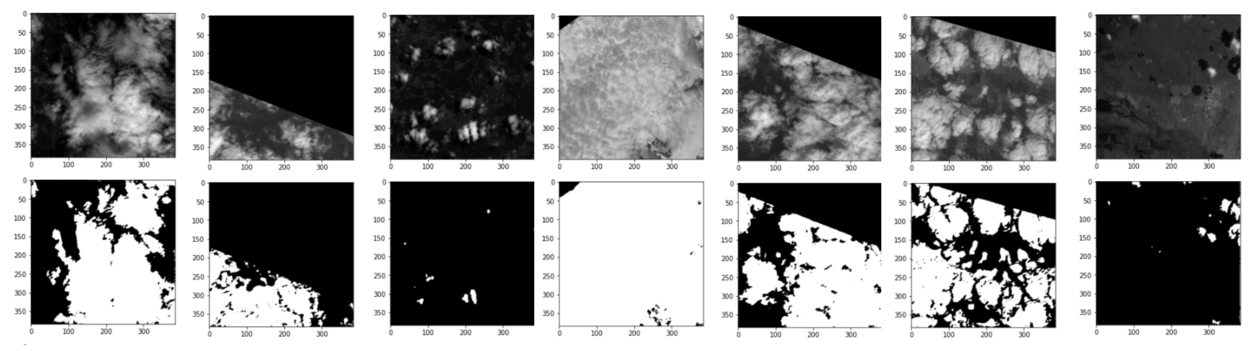
We see that the clouds are fairly well detected especially that we only trained for 20 epochs and only used 100 images.

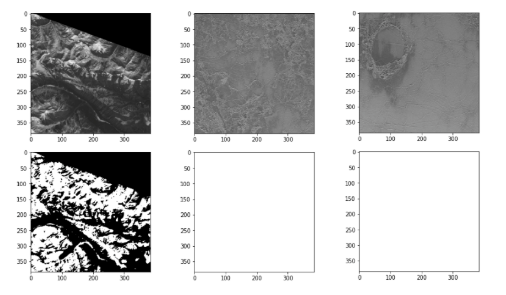
Some images are really challenging, for example, the top of a mountain with snow, or an empty landscape like a desert, is very confusing for the model. Indeed, the model might classify the snow on the top of a mountain as clouds, which would be a False Positive. We see this behavior with our trained model:

Detecting clouds on satellite images is an interesting and challenging problem, and now, you too can try to do it!

You can find the training notebook here!