Label Studio and Activeloop Hub. Work on semantic segmentation projects with a smile

In this tutorial, we will show how to make semantic segmentation projects easier using two computer vision tools: the open-source data labeling tool Label Studio and Hub, the dataset format for AI.

What is semantic segmentation?

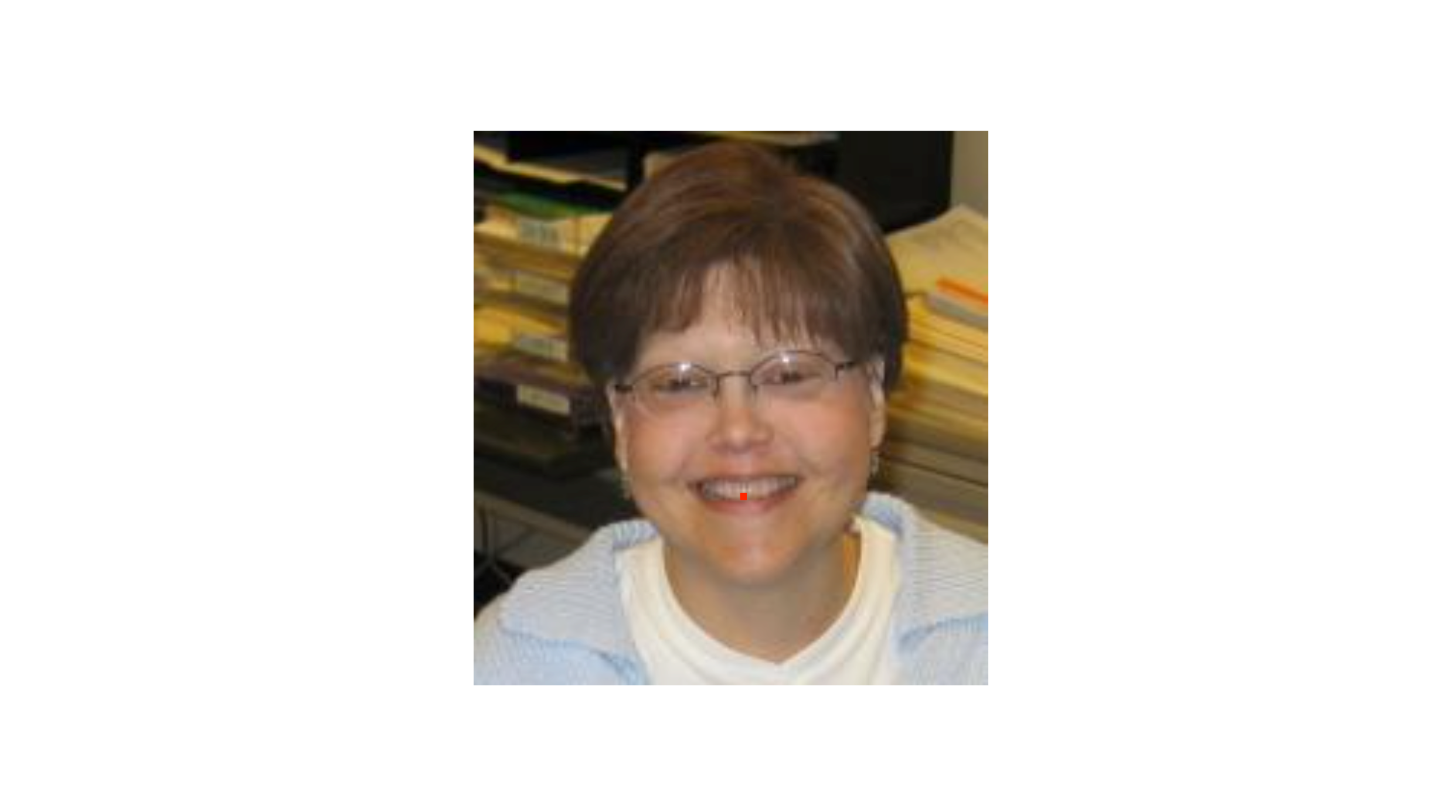
What is semantic segmentation? The goal of semantic segmentation is to attribute a class to each pixel of an image. In our case here, we want to know if a pixel belongs to the class “smile” or “non-smiling” so that we can know where the smile is on an image at the pixel level. For example, the red pixel on the image below belongs to the “smiling” class:

1) Image classification dataset GENKI-4K

So, for this project, we use the GENKI-4K subset that contains 4000 face images labeled as either “smiling” or “non-smiling” by human coders. We could use this labeling for image classification— is this image a picture of someone smiling or not? — but we want to segment the smiles, so we need to label the smiles on the actual images. Since we have the classification labeling, we can filter the images by only using the “smiling” images from the GENKI-4K subset.

First, we download the dataset from this link and select all the smiling images in the folder GENKI-R2009a/Subsets/GENKI-4K/files using the text files GENKI-4K_Labels.txt and GENKI-4K_Images.txt to know which images are labeled as “smiling” (smile=1, non-smile=0) in the labels text file, and each line is linked to the images’ names in the images text file.

2) Label Studio

Next, we will use Label Studio to label the smile on the images we’ve just gathered.

We chose to use the Docker installation for this so that we would not have to deal with any environment issues:

 
      

        
1docker run -it -p 8080:8080 -v `pwd`/mydata:/label-studio/data heartexlabs/label-studio:latest
2
        

          
            
            Copy
          
        
      
    

which will open the Label Studio web app at http://localhost:8080.

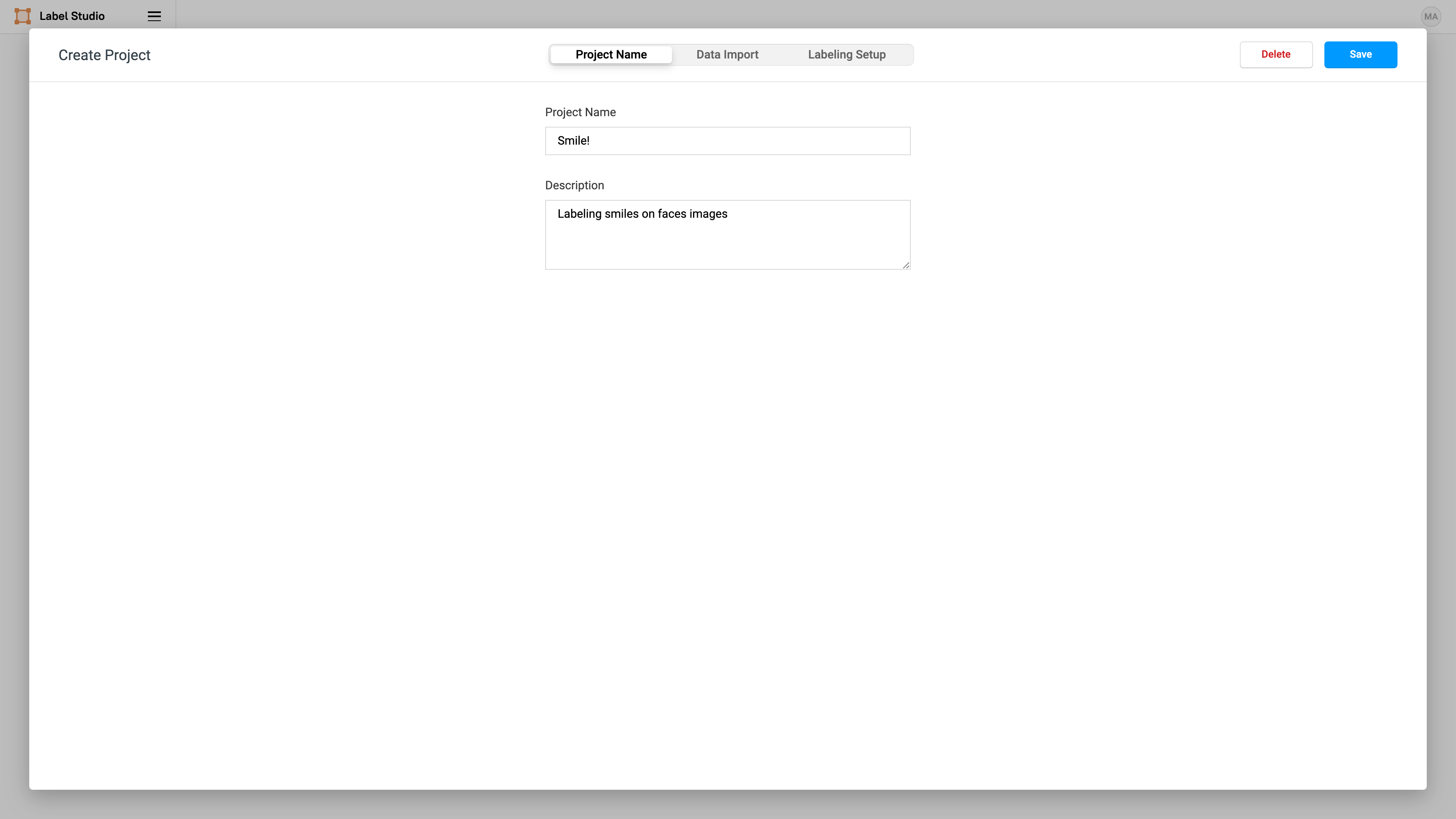
We sign up so that we can track who created the annotations, and then we can create our smile project! 😁

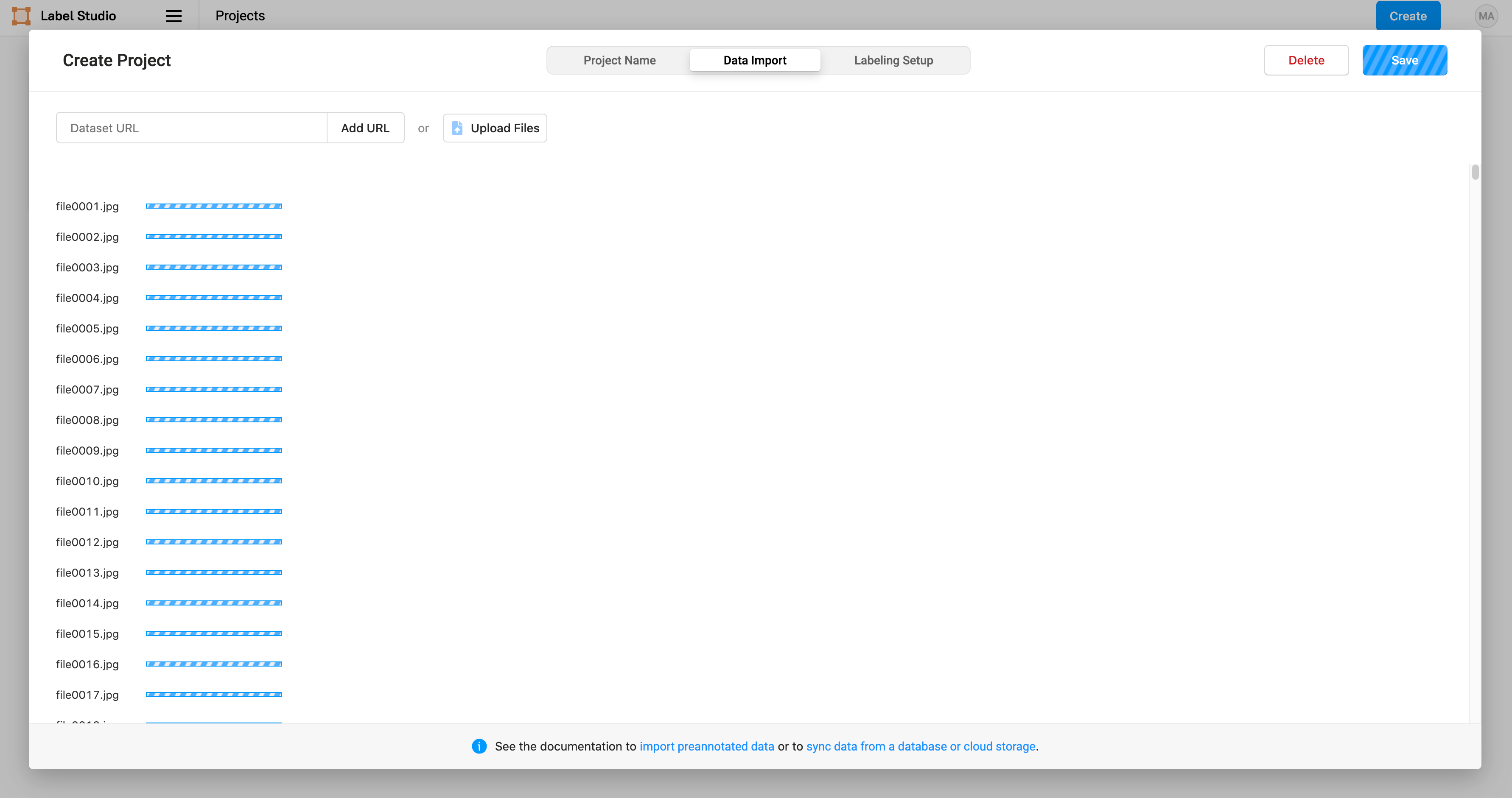
Then we import the smiling faces images selected from GENKI-4K:

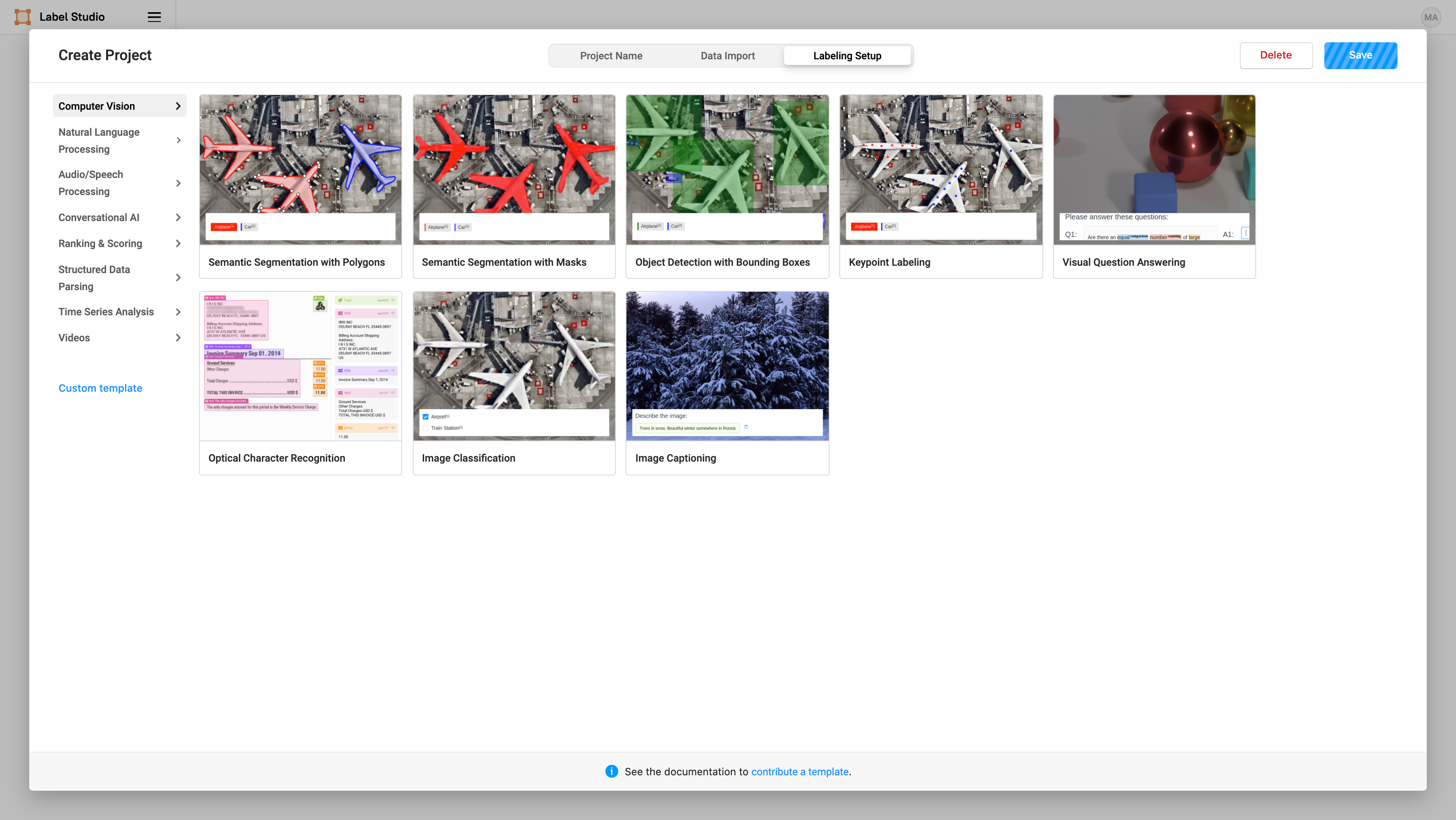
Label Studio makes it easy to perform a variety of computer vision labeling tasks. In this case, we select “Computer Vision” and “Semantic Segmentation with Masks” to use brush masks to highlight the smiles on images:

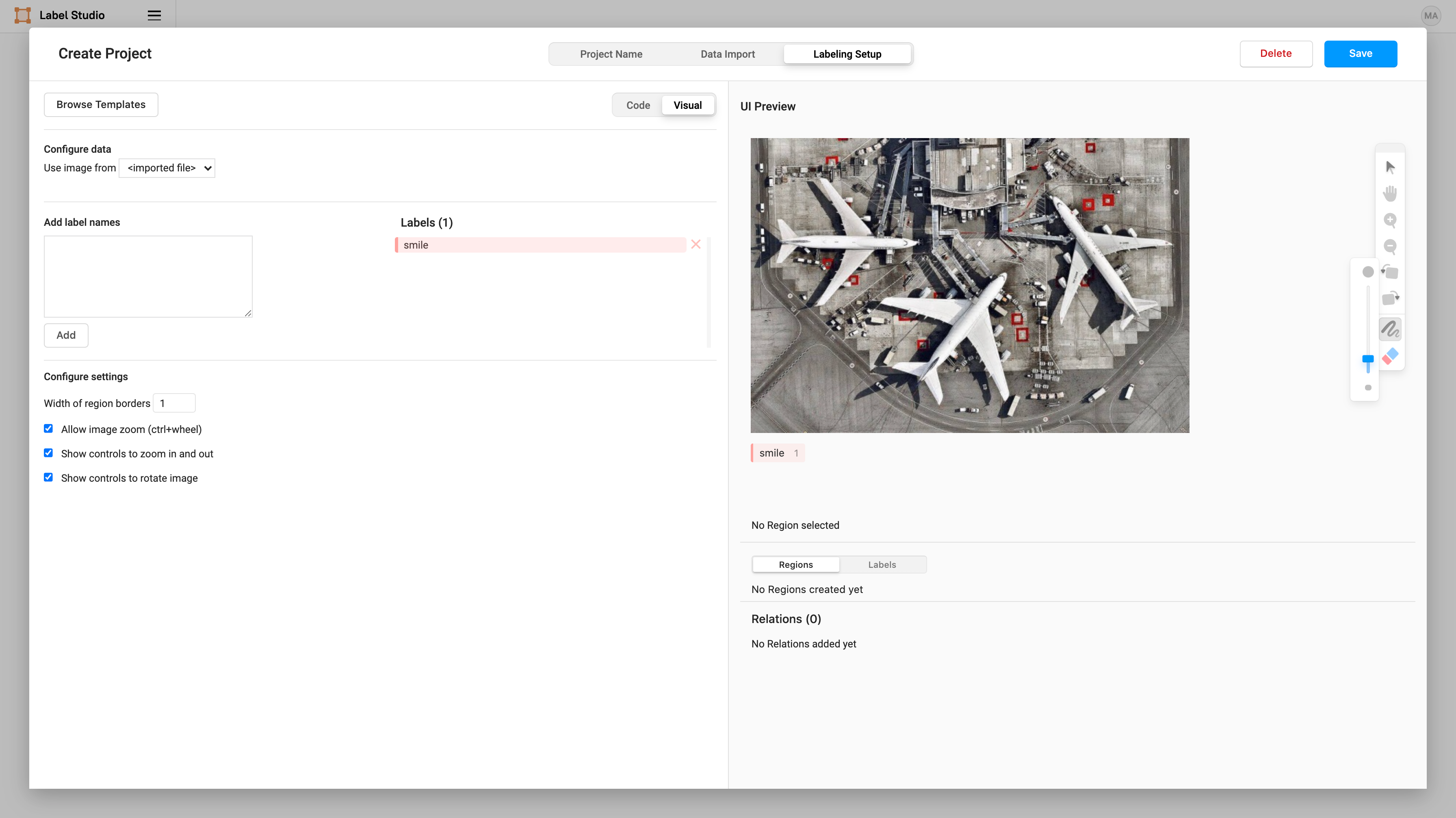
Then we can specify what label we want to assign to the brush masks that we create. Add a label name of “smile”.

Now we can start labeling smiles! 😬 (Labeling is the most time-consuming part of every computer vision — so be brave!).

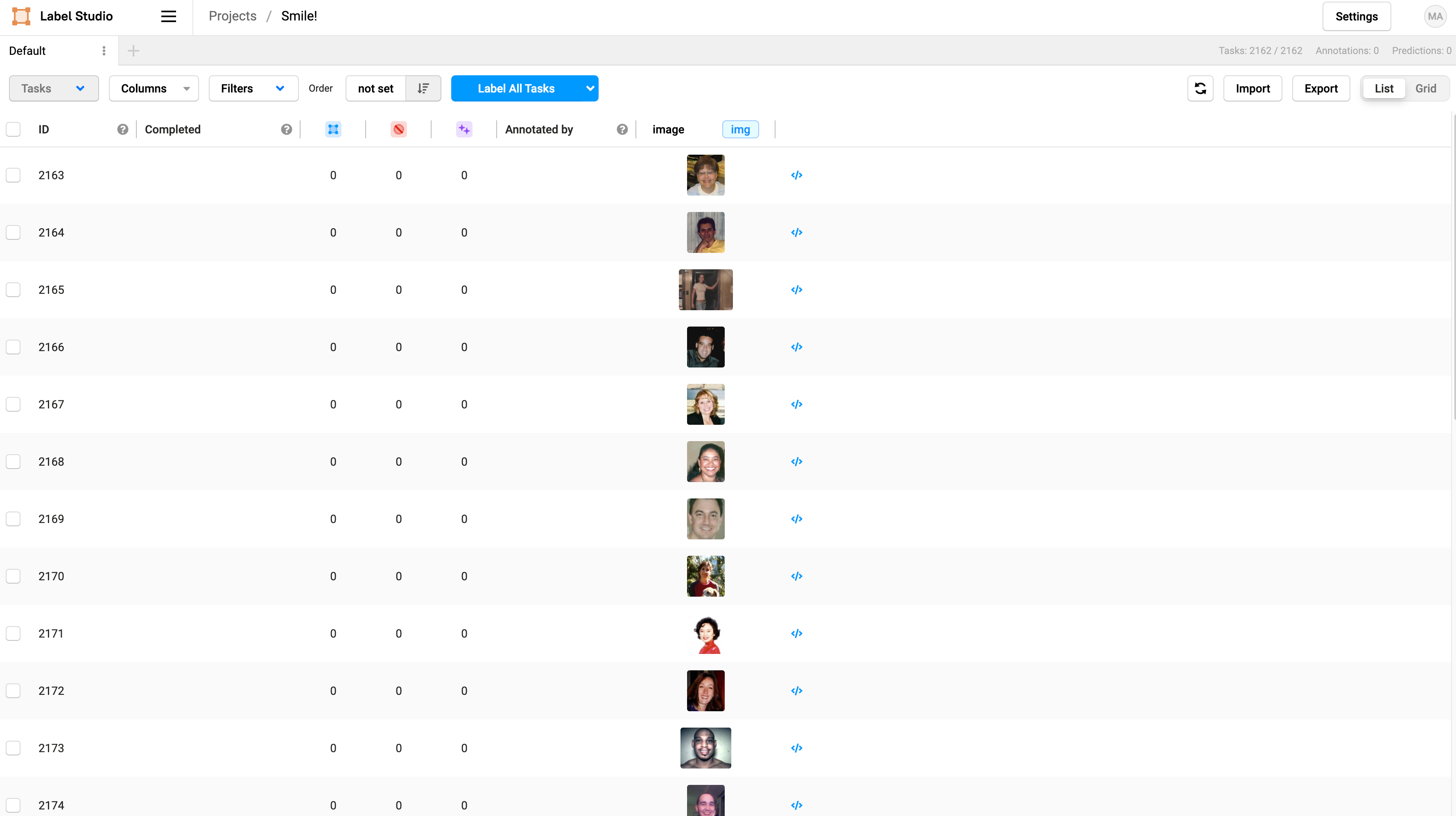
To start labeling, click on Label All Tasks. In this tutorial, we will only label 50 images, but you’d want to label at least 300 to get a reliably trained model for production.

We consider the “smile” to be the teeth and the mouth of the person so that we have a beautiful smiling shaped label 😃

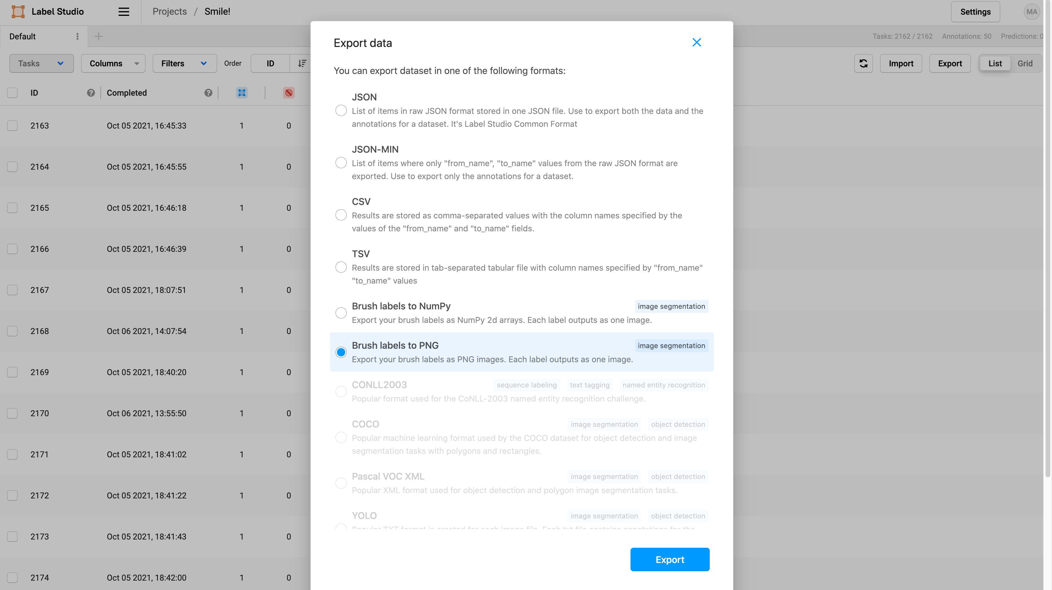
Once you are done labeling, you can export the images by clicking Export on the main page of your project, and then select Brush labels to PNG which will generate the labels as png files.

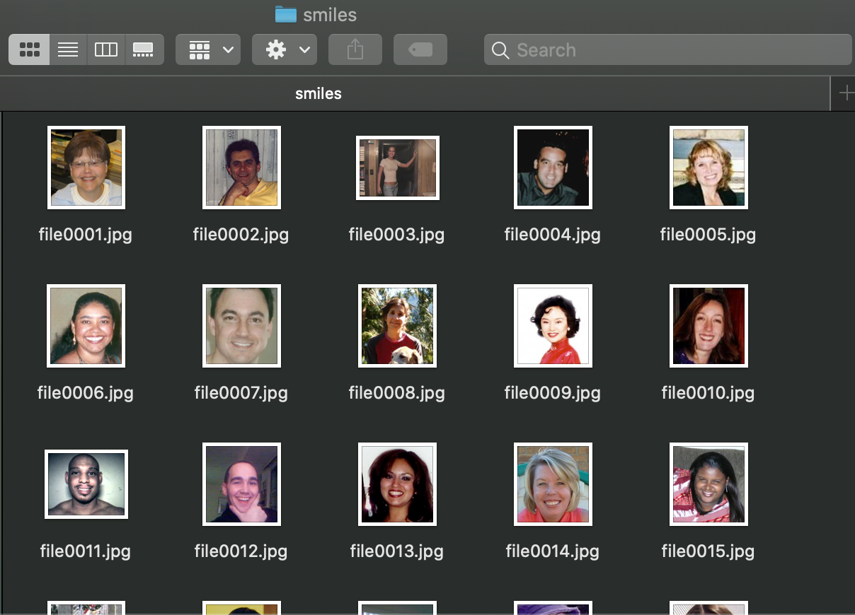
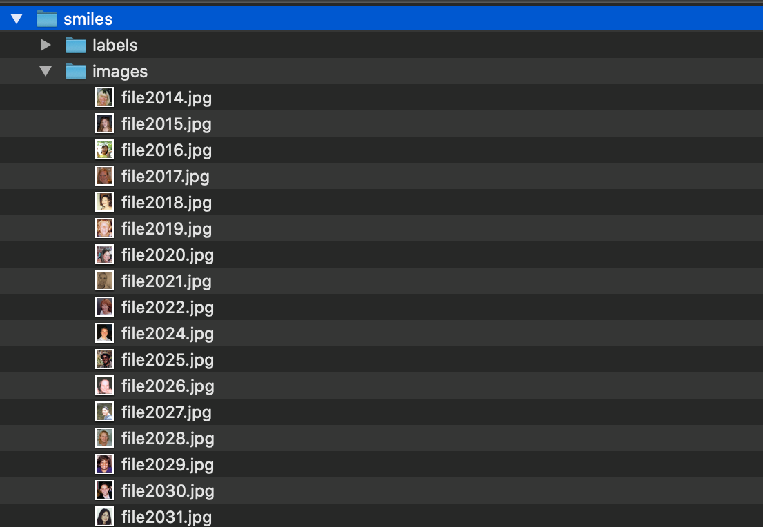
This will download a zipped folder with all the annotations. Unzip the folder and move the annotations png files under a subfolder called “labels” in a folder called “smiles” that already contains the smiling images from GENKI-4K.

Now, we can create a dataset and save it in Hub.

3) Create a computer vision dataset and send it to Hub Storage

We’ll create a dataset that you can easily and directly use to train a semantic segmentation model.

• Imports and visualization of the data

First, we install hub:

 
      

        
1pip install hub==2.0.11
2
        

          
            
            Copy
          
        
      
    

and import the packages we need for this step:

 
      

        
1import numpy as np
2import matplotlib.pyplot as plt
3import glob
4import cv2
5from tqdm import tqdm
6
        

          
            
            Copy
          
        
      
    

Let’s take a look at the images and masks we have:

 
      

        
1list_images = glob.glob('./images/*.jpg')
2list_images.sort()
3print(f'There are {len(list_images)} images')
4
        

          
            
            Copy
          
        
      
    

➡️ There are 2162 images

 
      

        
1list_masks = glob.glob('./labels/*.png')
2list_masks.sort()
3print(f'There are {len(list_masks)} masks')
4
        

          
            
            Copy
          
        
      
    

➡️ There are 50 masks

We visualize the first 10 images and their masks:

 
      

        
1for i in range(10):
2    img = cv2.cvtColor(cv2.imread(list_images[i]), cv2.COLOR_BGR2RGB)
3    print(f'Image shape: {img.shape}')
4
5mask = cv2.imread(list_masks[i], cv2.IMREAD_GRAYSCALE)
6    print(f'Mask shape: {mask.shape}')
7
8    plt.imshow(img)  
9    plt.show()
10
11    plt.imshow(mask, cmap="gray")  
12    plt.show()
13
        

          
            
            Copy
          
        
      
    

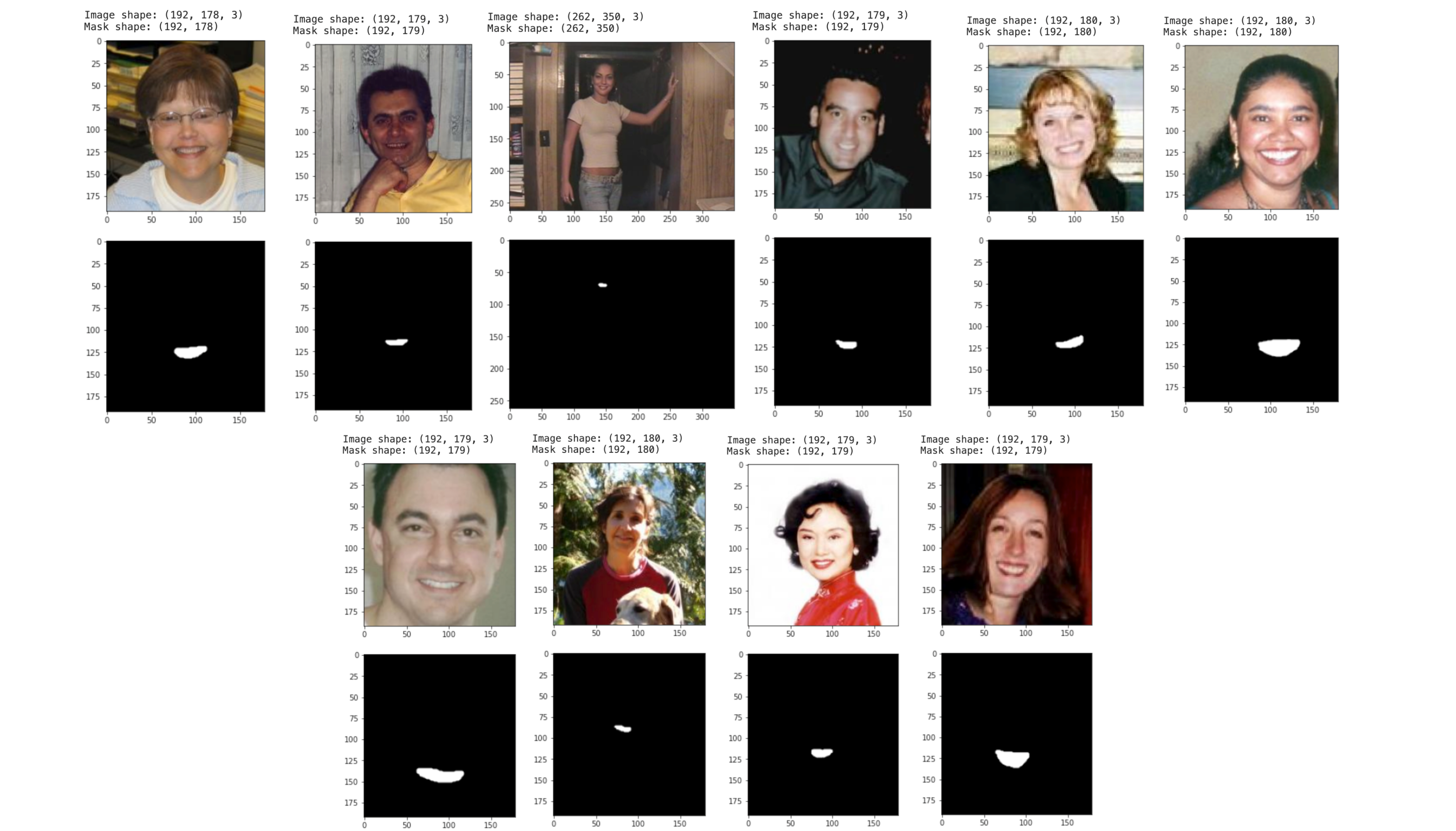
Everything looks good, so it’s time to send our images/masks to Hub!

• Upload data to Hub

You need to login to store a dataset in Hub:

 
      

        
1!activeloop login -u your_username -p your_password
2
        

          
            
            Copy
          
        
      
    

And we upload the dataset to Hub at the address hub://margauxmforsythe/smiles-segmentation:

 
      

        
1with hub.empty('hub://margauxmforsythe/smiles-segmentation', overwrite=True) as ds:
2    # Create the tensors with names of your choice.
3    ds.create_tensor('images', htype = 'image', sample_compression = 'jpg')
4    ds.create_tensor('masks', htype = 'image', sample_compression = 'png')
5
6   # Iterate through the files and append to hub dataset
7    for index in tqdm(range(len(list_masks))):
8        # Append to images tensor using hub.read
9        ds.images.append(hub.read(list_images[index]))
10
11        # Append to masks tensor using hub.read + Need to have 3 dimensions but only has 2 so we use np.expand_dims
12        ds.masks.append(np.expand_dims(hub.read(list_masks[index]), axis=2))
13
        

          
            
            Copy
          
        
      
    

Now, we can access this dataset with one line of code:

 
      

        
1ds = hub.dataset("hub://margauxmforsythe/smiles-segmentation")
2
        

          
            
            Copy
          
        
      
    

• Create test set with some of the non-labeled images and send it to Hub

We want to have some test images to run the our final model on that were not seen during the training. So, we select 100 images from the original non-labeled images:

 
      

        
1test_images_not_labeled = list_images[len(list_masks):len(list_masks)+100]
2
        

          
            
            Copy
          
        
      
    

and send those to Hub at the address hub://margauxmforsythe/smiles-segmentation-test:

 
      

        
1with hub.empty('hub://margauxmforsythe/smiles-segmentation-test', overwrite=True) as ds:
2    # Create the tensors with names of your choice.
3    ds.create_tensor('images', htype = 'image', sample_compression = 'jpg')
4
5    # Iterate through the files and append to hub dataset
6    for index in tqdm(range(len(test_images_not_labeled))):
7        # Append to images tensor using hub.read
8        ds.images.append(hub.read(test_images_not_labeled[index]))
9
        

          
            
            Copy
          
        
      
    

We have everything we need to start a training! 😃

You can find the notebook for uploading the data at this link.

4) Training: Say cheeeeese!

We are now training a semantic segmentation model (UNet).

First, we need to load our new smiling segmentation dataset from Hub:

 
      

        
1ds = hub.dataset("hub://margauxmforsythe/smiles-segmentation")
2
        

          
            
            Copy
          
        
      
    

and convert it to a Tensorflow dataset:

 
      

        
1ds_tf = ds.tensorflow()
2
        

          
            
            Copy
          
        
      
    

All images are not the same size, so we need to resize them, we chose a resize size of (256,256). We also need to make sure the values of the segmentation masks are binary (0 or 1) — which is not the case yet:

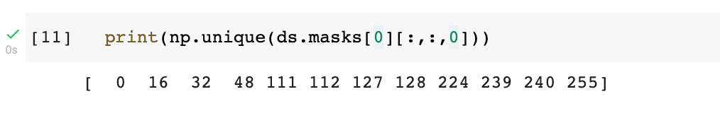
Indeed, here we see that there are other values that are not 0 or 1. We can fix this in the mapping function to_model_fit:

 
      

        
1resize_size = (256, 256)
2batch_size = 32
3
4def to_model_fit(item):
5    x = tf.image.resize(item['images'], resize_size)/255
6    y = item['masks']
7
8    # Need to have binary values: 0 or 1
9    y = tf.cast(y > 0, tf.int32)
10
11    # Resize
12    y = tf.image.resize(y, resize_size, method=tf.image.ResizeMethod.NEAREST_NEIGHBOR)
13    return (x, y)
14
15ds_tf = (ds_tf
16        # calling to_model_fit
17        .map(lambda item: to_model_fit(item))
18        .shuffle(len(ds))
19        .batch(batch_size)
20        .prefetch(tf.data.AUTOTUNE))
21
        

          
            
            Copy
          
        
      
    

NB: We shuffled, batched and prefetched the Tensorflow dataset at the same time as the mapping.

Now, we define the model we will use for this training:

 
      

        
1def unet(input_shape=(256, 256, 3)):
2    inputs = Input(input_shape)
3    conv1 = Conv2D(64, 3, activation = 'relu', padding = 'same', kernel_initializer = 'he_normal')(inputs)
4    conv1 = Conv2D(64, 3, activation = 'relu', padding = 'same', kernel_initializer = 'he_normal')(conv1)
5
6    pool1 = MaxPooling2D(pool_size=(2, 2))(conv1)
7    conv2 = Conv2D(128, 3, activation = 'relu', padding = 'same', kernel_initializer = 'he_normal')(pool1)
8    conv2 = Conv2D(128, 3, activation = 'relu', padding = 'same', kernel_initializer = 'he_normal')(conv2)
9
10    pool2 = MaxPooling2D(pool_size=(2, 2))(conv2)
11    conv3 = Conv2D(256, 3, activation = 'relu', padding = 'same', kernel_initializer = 'he_normal')(pool2)
12    conv3 = Conv2D(256, 3, activation = 'relu', padding = 'same', kernel_initializer = 'he_normal')(conv3)
13
14    pool3 = MaxPooling2D(pool_size=(2, 2))(conv3)
15    conv4 = Conv2D(512, 3, activation = 'relu', padding = 'same', kernel_initializer = 'he_normal')(pool3)
16    conv4 = Conv2D(512, 3, activation = 'relu', padding = 'same', kernel_initializer = 'he_normal')(conv4)
17
18    drop4 = Dropout(0.5)(conv4)
19    pool4 = MaxPooling2D(pool_size=(2, 2))(drop4)
20
21    conv5 = Conv2D(1024, 3, activation = 'relu', padding = 'same', kernel_initializer = 'he_normal')(pool4)
22    conv5 = Conv2D(1024, 3, activation = 'relu', padding = 'same', kernel_initializer = 'he_normal')(conv5)
23    drop5 = Dropout(0.5)(conv5)
24
25    up6 = Conv2D(512, 2, activation = 'relu', padding = 'same', kernel_initializer = 'he_normal')(UpSampling2D(size = (2,2))(drop5))
26    merge6 = concatenate([drop4,up6], axis = 3)
27    conv6 = Conv2D(512, 3, activation = 'relu', padding = 'same', kernel_initializer = 'he_normal')(merge6)
28    conv6 = Conv2D(512, 3, activation = 'relu', padding = 'same', kernel_initializer = 'he_normal')(conv6)
29
30    up7 = Conv2D(256, 2, activation = 'relu', padding = 'same', kernel_initializer = 'he_normal')(UpSampling2D(size = (2,2))(conv6))
31    merge7 = concatenate([conv3,up7], axis = 3)
32    conv7 = Conv2D(256, 3, activation = 'relu', padding = 'same', kernel_initializer = 'he_normal')(merge7)
33    conv7 = Conv2D(256, 3, activation = 'relu', padding = 'same', kernel_initializer = 'he_normal')(conv7)
34
35    up8 = Conv2D(128, 2, activation = 'relu', padding = 'same', kernel_initializer = 'he_normal')(UpSampling2D(size = (2,2))(conv7))
36    merge8 = concatenate([conv2,up8], axis = 3)
37    conv8 = Conv2D(128, 3, activation = 'relu', padding = 'same', kernel_initializer = 'he_normal')(merge8)
38    conv8 = Conv2D(128, 3, activation = 'relu', padding = 'same', kernel_initializer = 'he_normal')(conv8)
39
40    up9 = Conv2D(64, 2, activation = 'relu', padding = 'same', kernel_initializer = 'he_normal')(UpSampling2D(size = (2,2))(conv8))
41    merge9 = concatenate([conv1,up9], axis=3)
42    conv9 = Conv2D(64, 3, activation = 'relu', padding = 'same', kernel_initializer = 'he_normal')(merge9)
43
44    conv10 = Conv2D(1, 1, activation='sigmoid')(conv9)
45
46    model = Model(inputs=inputs, outputs=conv10)
47
48    return model
49
        

          
            
            Copy
          
        
      
    

We initialize the model:

 
      

        
1model = unet((256,256,3))
2
        

          
            
            Copy
          
        
      
    

And compile it with a set of useful metrics for semantic segmentation:

 
      

        
1model.compile(optimizer=tf.keras.optimizers.Adam(0.0001), 
2              loss='binary_crossentropy',
3              metrics=[tf.keras.metrics.BinaryAccuracy(), tf.keras.metrics.Recall(name="recall"), 
4                       tf.keras.metrics.Precision(name="precision")])
5
        

          
            
            Copy
          
        
      
    

We define the callbacks we will use when training the model:

 
      

        
1# Early Stopping Callback
2early_stop = tf.keras.callbacks.EarlyStopping(
3    monitor='loss', patience=21, verbose=1,
4    mode='min', restore_best_weights=True
5)
6
7# Reduce learning rate callback
8reduce_lr = tf.keras.callbacks.ReduceLROnPlateau(
9    monitor="loss",
10    factor=0.1,
11    patience=10,
12    verbose=1,
13    mode="min",
14)
15
        

          
            
            Copy
          
        
      
    

and we train the model for 200 epochs:

 
      

        
1model.fit(ds_tf, epochs = 200, callbacks=[early_stop, reduce_lr])
2
        

          
            
            Copy
          
        
      
    

Once this is done training, we use this model on our test set:

 
      

        
1# Load from Hub
2ds_test = hub.dataset("hub://margauxmforsythe/smiles-segmentation-test")
3
4# Convert it to Tensorflow dataset, we decide to use a batch size of 1 for this test set
5def to_model_fit(item):
6    x = tf.image.resize(item['images'], resize_size)/255
7    return (x)
8
9ds_test_tf = ds_test.tensorflow()
10
11ds_test_tf = (ds_test_tf
12            .map(lambda item: to_model_fit(item))
13            .batch(1))
14
        

          
            
            Copy
          
        
      
    

and finally, we gather the predictions in the variable results:

 
      

        
1# Run the inference on the test set
2results = model.predict(ds_test_tf)
3
        

          
            
            Copy
          
        
      
    

We select a probabilities threshold of 0.8, which means that the pixels where probabilities in results > threshold_probabilities will be accounted as “smiling” pixels.

 
      

        
1threshold_probabilities = 0.8
2
3i = 0 
4for image in ds_test_tf:
5  plt.imshow(image[0]) # index = 0 because we set batchsize of test dataset to 1
6  plt.show()
7  pred = (results[i][:,:,0] > threshold_probabilities).astype(np.uint8)
8  plt.imshow(pred, cmap="gray")
9  plt.show()
10  print(np.unique(pred))
11  i = i + 1
12  if i > 10:
13    break
14
        

          
            
            Copy
          
        
      
    

Results:

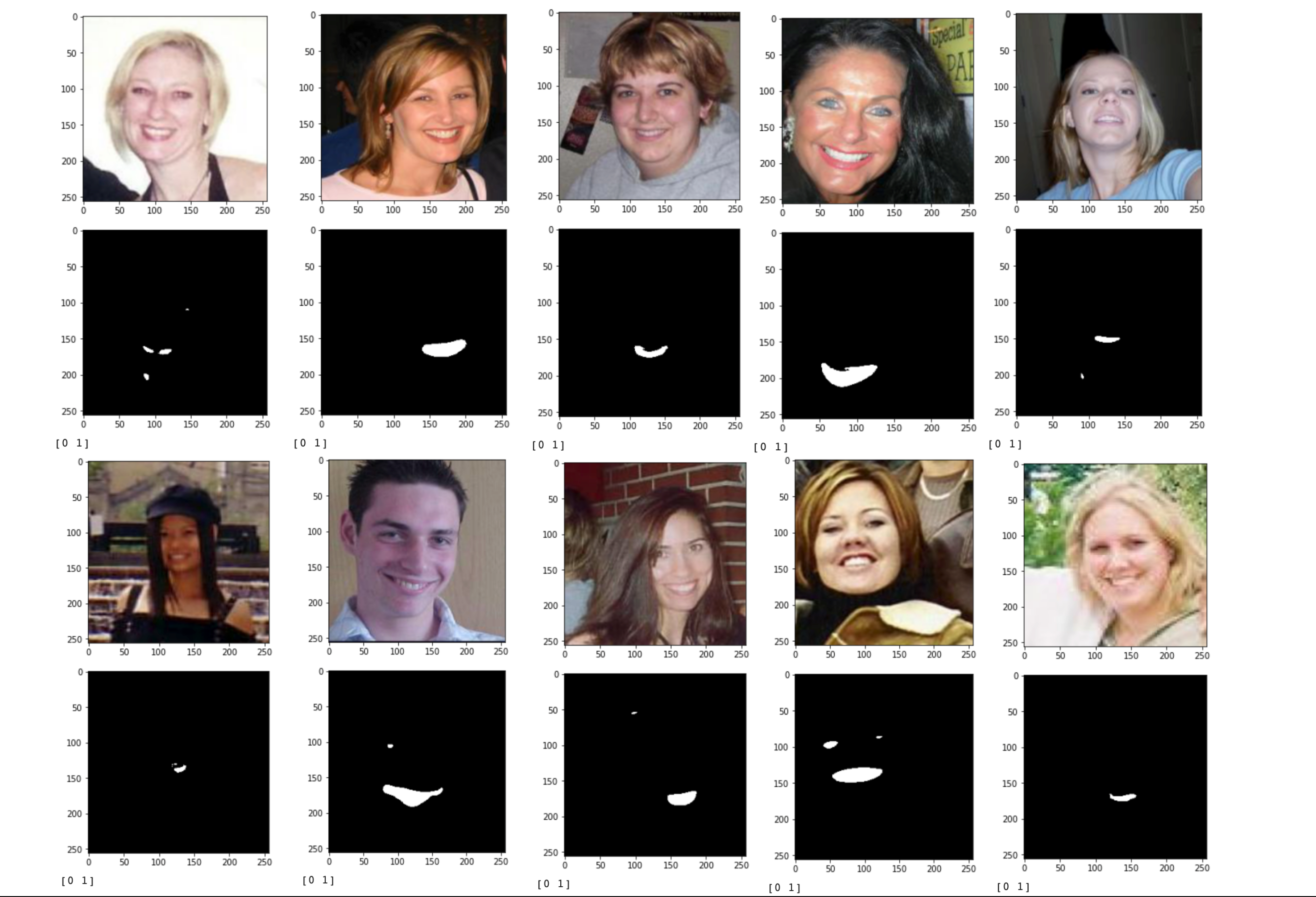
Done! Of course, we need more labeling and hyperparameters optimization in order to have better results 🙃 Share your results with us if you try this out!

The training notebook for this tutorial is here.