Introduction

The workflow of a Machine Learning (ML) project includes all the stages required to put in production a model that performs a task such as image classification. The figure below gives a high-level overview of these stages:

If you are familiar with Machine Learning workflow, you probably know that the most time-expensive step is — most of the time — the Data Preparation one. There are several reasons why this step takes up a lot of time:

• Working with real-world data is complex and often requires a lot of cleaning

• Data-preprocessing algorithms are often slow which exponentially gets worse when the amount of data increases, or if the pre-processing steps have to be re-run for some reasons

• Choosing the optimal data storage solution is not easy and can be quite expensive

• Sharing data with the rest of the team is harder than sharing code

In this article, we will analyze the time that it takes to perform an easy task from the data preparation stage: Uploading a dataset to the Cloud that can be shared with others. For this, we will compare how long it takes the send a computer vision dataset to an Amazon Web Service (AWS) s3 bucket versus sending it to Hub.

Benchmark study: Uploading a dataset to the Cloud

Most ML teams use Cloud storage to store and access data. Especially when working on computer vision projects, the datasets can get really heavy and are hard to store locally. Some companies use a NAS (Network Attached Storage) to store their data but, in the past couple of years, a lot of them are starting to switch to Cloud storage instead. It is indeed much easier not to have to deal with configuring and maintaining an on-growing NAS.

So, which is the fastest between s3 or Hub?

For this comparison, we chose to use the Kaggle dataset: A Large-Scale Dataset for Fish Segmentation and Classification.

1. Download the Dataset

First, let’s download the dataset from Kaggle using this command:

export KAGGLE_USERNAME="xxxxxx" && export KAGGLE_KEY="xxxxxx" && kaggle datasets download -d crowww/a-large-scale-fish-dataset

This will download the archived dataset in the workspace, and now need to be unzipped:

unzip -n a-large-scale-fish-dataset.zip

The dataset is organized by subfolders that each corresponds to a class (fish species):

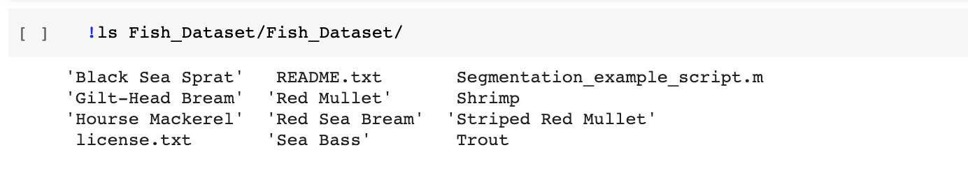
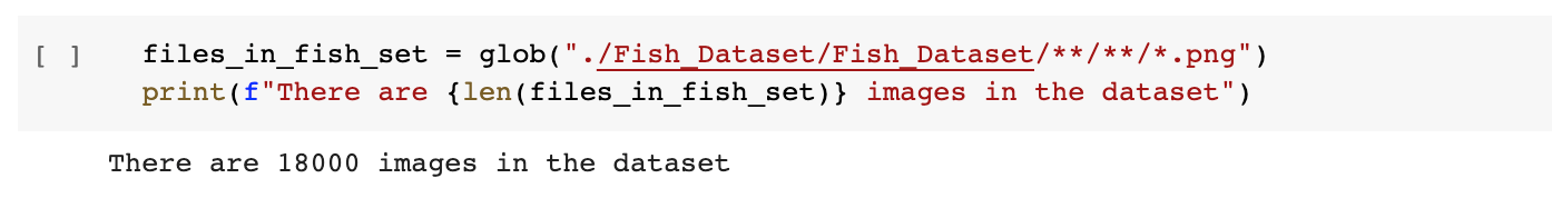
This dataset is quite large, in total, we have 18000 png images. Each fish species subfolder has two subfolder: one that contains the RGB images of the fished and one that contains the corresponding segmentation mask (also called the GT=Ground Truth).

We gather all the paths to the images in a list called files_in_fish_set_images and all the paths to the masks the list files_in_fish_set_GT:

import fnmatch

files_in_fish_set_images = []
files_in_fish_set_GT = []
for dirpath, dirs, files in os.walk(dataset_path): 
  for filename in fnmatch.filter(files, '*.png'):
    fname = os.path.join(dirpath,filename)
    if 'GT' in fname:
      files_in_fish_set_GT.append(fname)
    else:
      files_in_fish_set_images.append(fname)

print(f'There are {len(files_in_fish_set_images)} pictures of fish and {len(files_in_fish_set_GT)} corresponding masks (GT)')

➡️ There are 9000 pictures of fish and 9000 corresponding masks (GT)

So we have 18000 images in total, with half of them that are pictures of fished and the other half, the corresponding segmentation masks.

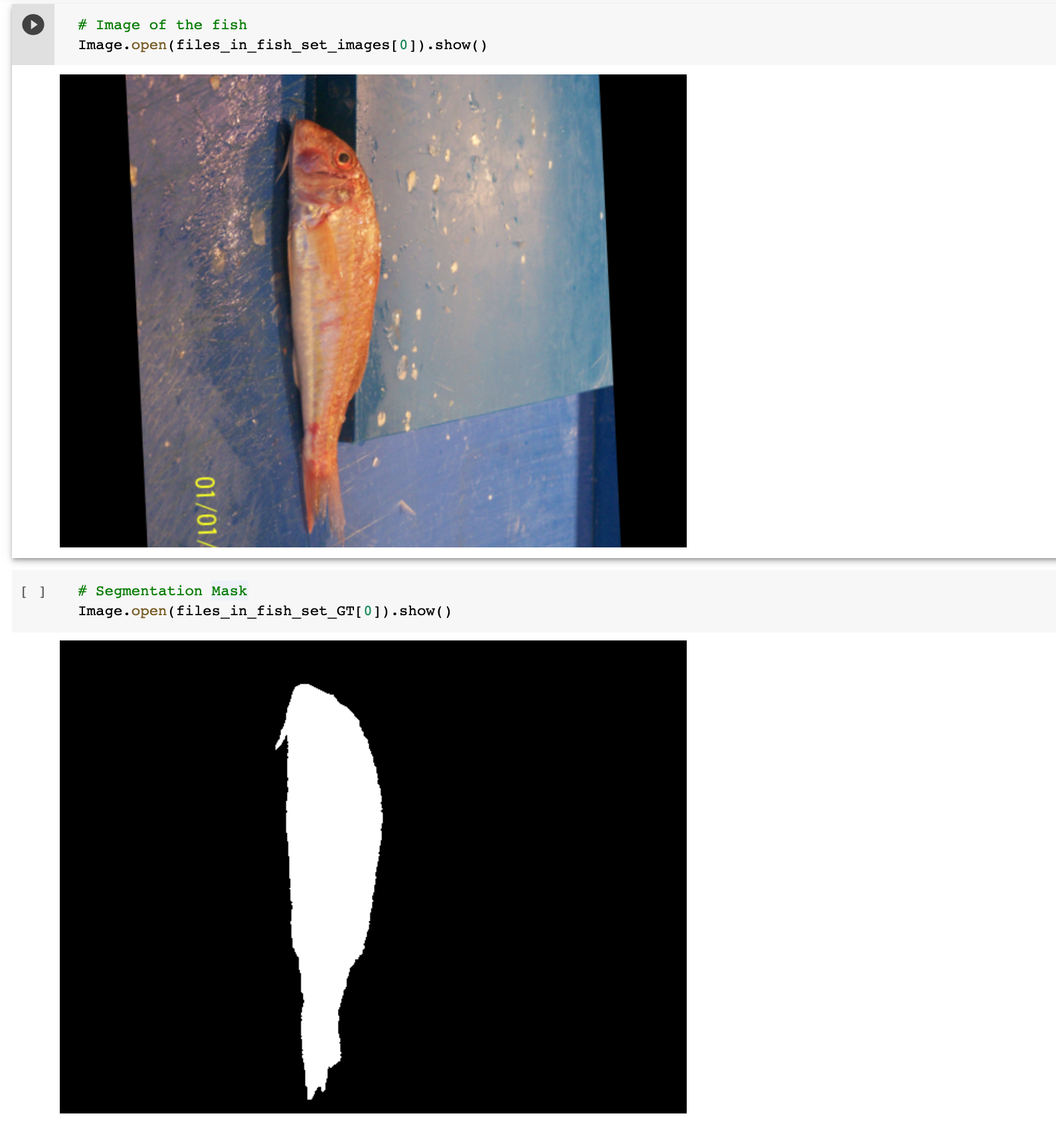
We visualized the first pair image/mask in the dataset, using the Image package from Pillow:

from PIL import Image

2. Send dataset to s3 bucket: AWS CLI

We are sending the dataset to the s3 bucket first. We will use AWS Command Line Interface (AWS CLI) to perform this task, so let’s install this package using pip:

# Install AWS CLI 
!pip install --upgrade awscli

Then you need to set up your AWS credentials:

# Congigure AWS credentials 
!aws configure

In order to send the ASL dataset to the s3 bucket using this command:

# Send dataset to s3 using aws CLI
# We created a bucket "fish-classification-segmentation-dataset" in s3 ahead of time
!aws s3 cp --recursive --no-progress --only-show-errors "./Fish_Dataset" "s3://fish-classification-segmentation-dataset"

But we also want to evaluate the time that this command will take so we set up a timer that starts before running this line and stops at the end of the execution of this task:

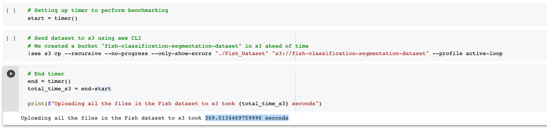
➡️ Sending the dataset to s3 using AWS CLI took ~370 seconds.

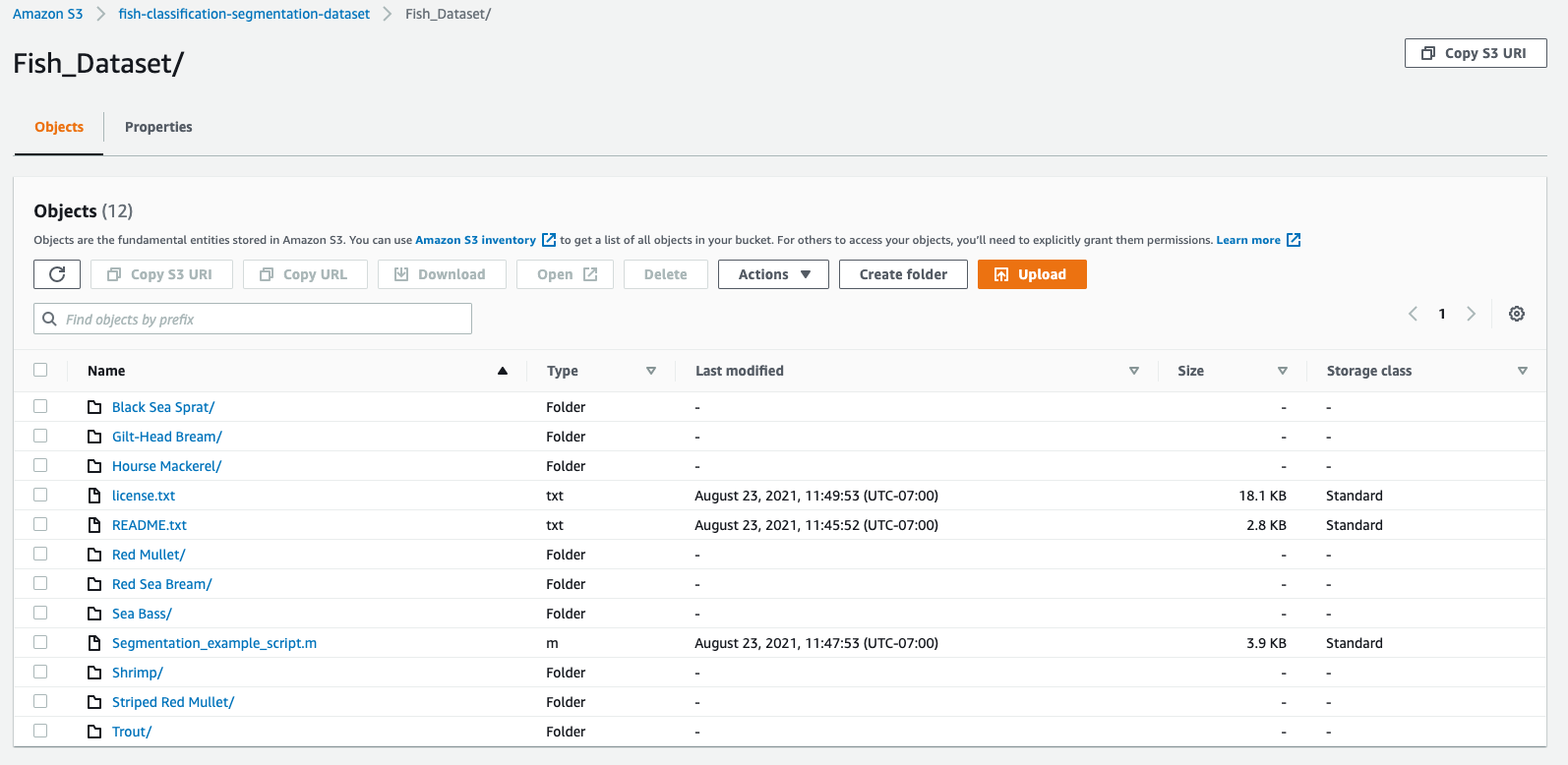
Then, if we check in our s3 bucket, we do see all the subfolders were uploaded:

3. Send dataset to s3 bucket: boto3

Now we will test with a pretty commonly used package to communicate with AWS s3 called boto3.

We need to import the following packages:

import boto3
from botocore.exceptions import NoCredentialsError
from timeit import default_timer as timer
from tqdm import tqdm

Then we set up our AWS credentials variables:

ACCESS_KEY = 'xxxxxx'
SECRET_KEY = 'xxxxxx'
AWS_SESSION_TOKEN='xxxxxx'

Now we can use these credentials to connect to s3 using boto3.client:

# Set up connection to s3 account with credentials provided by user
s3_client = boto3.client('s3', aws_access_key_id=ACCESS_KEY,
                          aws_secret_access_key=SECRET_KEY, 
                          aws_session_token=AWS_SESSION_TOKEN)

We then implement the function upload_to_aws that sends a file to an s3 bucket. It takes as inputs: the s3 client we just configured, the path to the local file to send to s3, the name of the s3 bucket we want the file to be sent to, and the name we want the file to be named in the s3 bucket:

def upload_to_aws(s3_client, local_file, bucket, s3_file):
    # Try to upload file to s3 bucket and handle errors that can happens. 
    # Returns True if success, False otherwise
    try:
        s3_client.upload_file(local_file, bucket, s3_file)
        print("Upload Successful")
        return True
    except FileNotFoundError:
        print("The file was not found")
        return False
    except NoCredentialsError:
        print("Credentials not available")
        return False

As said before, this function sends only one file to the s3 bucket, so we need to implement a loop that goes through all of the images in the dataset, and sends them to s3 — and we will also add a timer to log how much time this whole process took — so that we can then compare this time to the other times:

# We created a bucket in s3 called fish-classification-segmentation-dataset-boto3
bucket_name = "fish-classification-segmentation-dataset-boto3"

# Setting up timer to perform benchmarking
start = timer()

for img_path in tqdm(files_in_fish_set):
  # We only want the file's name after "./Fish_Dataset/Fish_Dataset/"
  file_name_in_s3 = img_path.split(dataset_path)[1]
  # Upload file to the bucket 
  uploaded = upload_to_aws(s3_client, img_path, bucket_name, file_name_in_s3)

# End timer
end = timer()
total_time_s3 = end-start

print(f"Uploading all the files in the Fish dataset to s3 took {total_time_s3} seconds")

And this is the result:

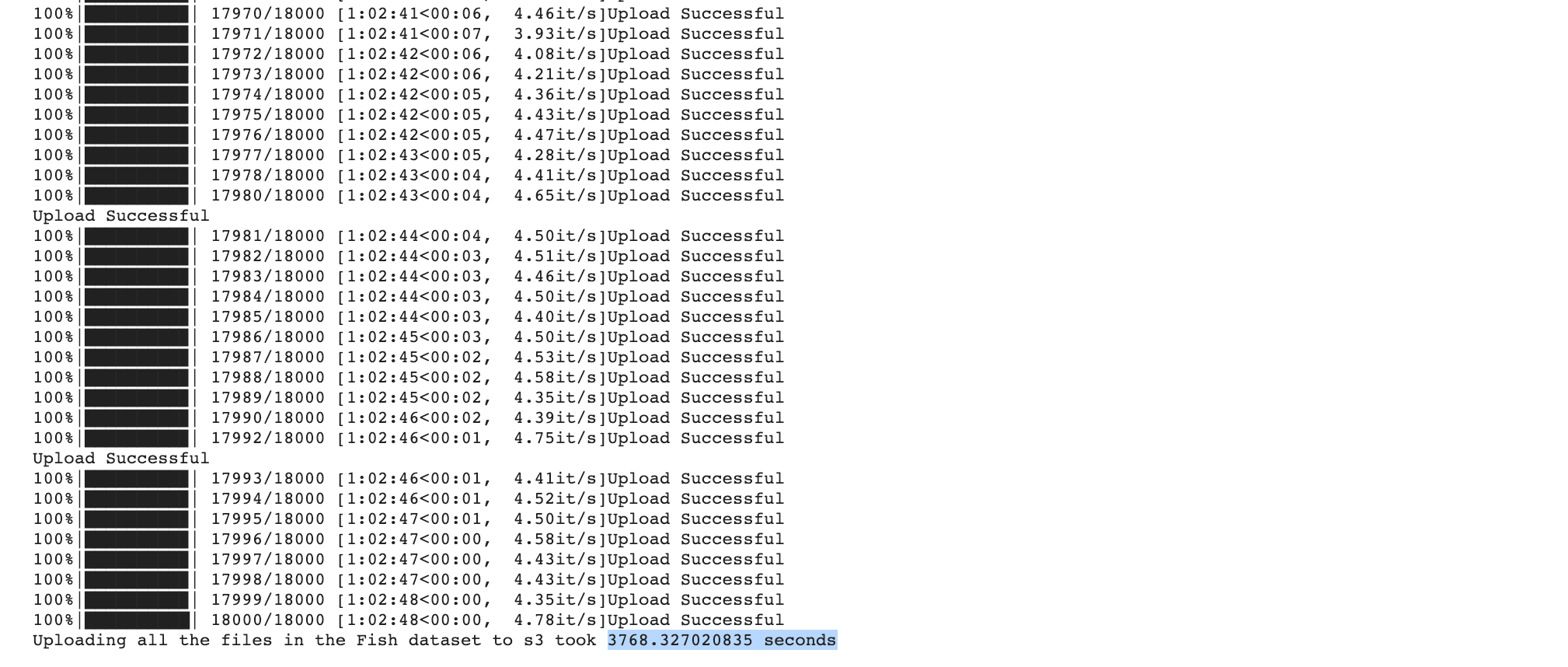
➡️ Uploading all the files in the Fish dataset with boto3 to s3 took 3768.327020835 seconds.

The script took approximately 63 minutes to execute. We can see here that using AWS CLI is much faster than boto3.

Now, we can try to send the zipped dataset to s3 using boto3:

# Upload the zipped dataset
# Setting up timer to perform benchmarking
start = timer()

path_to_zipped_dataset = 'a-large-scale-fish-dataset.zip'
uploaded = upload_to_aws(s3_client, path_to_zipped_dataset, bucket_name, path_to_zipped_dataset)

# End timer
end = timer()
total_time_s3 = end-start

print(f"Uploading the zipped Fish dataset to s3 took {total_time_s3} seconds")

Result:

➡️ Sending the zipped dataset to s3 using boto3 took 40.643983771999956 seconds.

This is a good way to send the zipped dataset to s3, however, the user will have to download and unzip the dataset each time they want to use or visualize it from the s3 bucket.

4. Send dataset to Hub

Now let’s send the dataset to Hub. First, here is how you can install Hub with pip:

pip install hub==2.0.7

NB: if using Google Colab, restart the runtime after running this line.

Then, we import the modules we will need:

import hub
import numpy as np

We also need to login to Activeloop:

!activeloop login -u username -p password

We are using the Hub storage, so we define a Hub path to the dataset that we are about to create and populate:

hub_fish_path = "hub://margauxmforsythe/fish-dataset"

We need to know the names of all the classes in the dataset so that they can be configured as labels in the Hub dataset:

# Find the class_names 
# we do not want the txt files to be included so we only look for the subfolders' names
class_names = [name for name in os.listdir(dataset_path) if os.path.isdir(dataset_path + name)]

print(f"There are {len(class_names)} classes: {class_names}")

➡️ There are 9 classes: [‘Striped Red Mullet’, ‘Black Sea Sprat’, ‘Trout’, ‘Hourse Mackerel’, ‘Shrimp’, ‘Sea Bass’, ‘Red Mullet’, ‘Gilt-Head Bream’, ‘Red Sea Bream’]

So we have the 9 different species of fish.

We can now send the dataset to Hub (i.e. in Hub format to Activeloop Cloud). In this dataset, each item will have an image, a mask and a label. And once again, we will use a timer to know how much time this command took so that we can compare it to the previous tests:

# Setting up timer to perform benchmarking
start = timer()

# Uploading to Hub storage at the path: hub_asl_path
with hub.empty(hub_fish_path, overwrite=True) as ds:
    # Create the tensors with names of your choice.
    ds.create_tensor('images', htype = 'image', sample_compression = 'png')
    ds.create_tensor('masks', htype = 'image', sample_compression = 'png')
    ds.create_tensor('labels', htype = 'class_label', class_names = class_names)

    # Add arbitrary metadata - Optional
    ds.info.update(description = 'Fish classification & Segmentation dataset')
    ds.images.info.update(camera_type = 'SLR')

    # Iterate through the files and append to hub dataset
    for i in tqdm(range(len(files_in_fish_set_images))):
        file_image = files_in_fish_set_images[i]
        file_mask = files_in_fish_set_GT[i]
        label_text = os.path.basename(os.path.dirname(file_image))
        label_num = class_names.index(label_text)

        # Append to images tensor using hub.read
        ds.images.append(hub.read(file_image))  
        # Append to masks tensor using hub.read
        ds.masks.append(hub.read(file_mask))  
        # Append to labels tensor
        ds.labels.append(np.uint32(label_num)) 

# End timer
end = timer()
total_time_hub = end-start

print(f"Uploading all the files in the Fish dataset to Hub took {total_time_hub} seconds")

➡️ Uploading all the files in the Fish dataset to Hub took 1047.8884124840006 seconds.

This took quite a long time. However, with Hub, we can use parallel computing to upload a dataset faster. Let’s try it!

First, we implement the function file_to_hub that will run in parallel and that converts data from files (image, mask, label) into hub format:

@hub.compute
def file_to_hub(path_to_pair_img_mask, sample_out, class_names):
    file_image = path_to_pair_img_mask[0]
    file_mask = path_to_pair_img_mask[1]

    label_text = os.path.basename(os.path.dirname(file_image))
    label_num = class_names.index(label_text)

    # Append the label and image to the output sample
    sample_out.labels.append(np.uint32(label_num))
    sample_out.images.append(hub.read(file_image))
    sample_out.masks.append(hub.read(file_mask))

    return sample_out

We defined file_to_hub such as it takes as input a list with two items: the path to the image and the path to the corresponding mask. Therefore, we need to create this list to be able to populate our dataset:

# Creating a list that combined the paths to the pairs image/mask 
list_pairs_img_mask = [[files_in_fish_set_images[i], files_in_fish_set_GT[i]] for i in range(len(files_in_fish_set_images))]

So now we have the list list_pairs_img_mask that contains the paths to all the pairs image/mask, for example here is the first item of the list:

list_pairs_img_mask[0]= [‘./Fish_Dataset/Fish_Dataset/Striped Red Mullet/Striped Red Mullet/00361.png’,
 ‘./Fish_Dataset/Fish_Dataset/Striped Red Mullet/Striped Red Mullet GT/00361.png’]

We are ready to create our new dataset that we will call hub_fish_path_parallel_computing, available at the path ‘hub://margauxmforsythe/fish_dataset_parallel_computing’ using parallel computing (for this example, we use num_workers = 10 which should really speed up the process):

hub_fish_path_parallel_computing = 'hub://margauxmforsythe/fish_dataset_parallel_computing'

# Setting up timer to perform benchmarking
start = timer()

with hub.empty(hub_fish_path_parallel_computing, overwrite=True) as ds:
    ds.create_tensor('images', htype = 'image', sample_compression = 'png')
    ds.create_tensor('masks', htype = 'image', sample_compression = 'png')
    ds.create_tensor('labels', htype = 'class_label', class_names = class_names)

    file_to_hub(class_names=class_names).eval(list_pairs_img_mask, ds, num_workers = 10)

# End timer
end = timer()
total_time_hub = end-start

print(f"Uploading all the files in the Fish dataset to Hub with parallel computing took {total_time_hub} seconds")

➡️ It only took 182.68960309999966 seconds to upload the Fish dataset to Hub when using parallel computing!

Let’s take a look at our dataset:

ds_from_hub_parallel_computing = hub.dataset(hub_fish_path_parallel_computing)

list_random = [random.randint(0,len(ds_from_hub)) for i in range(8)]

for i in list_random:
  print(f'\n{class_names[ds_from_hub_parallel_computing.labels[i].numpy()[0]]}')
  Image.fromarray(ds_from_hub_parallel_computing.images[i].numpy()).show()

  # grayscale mask
  Image.fromarray(ds_from_hub_parallel_computing.masks[i].numpy()*255).show()

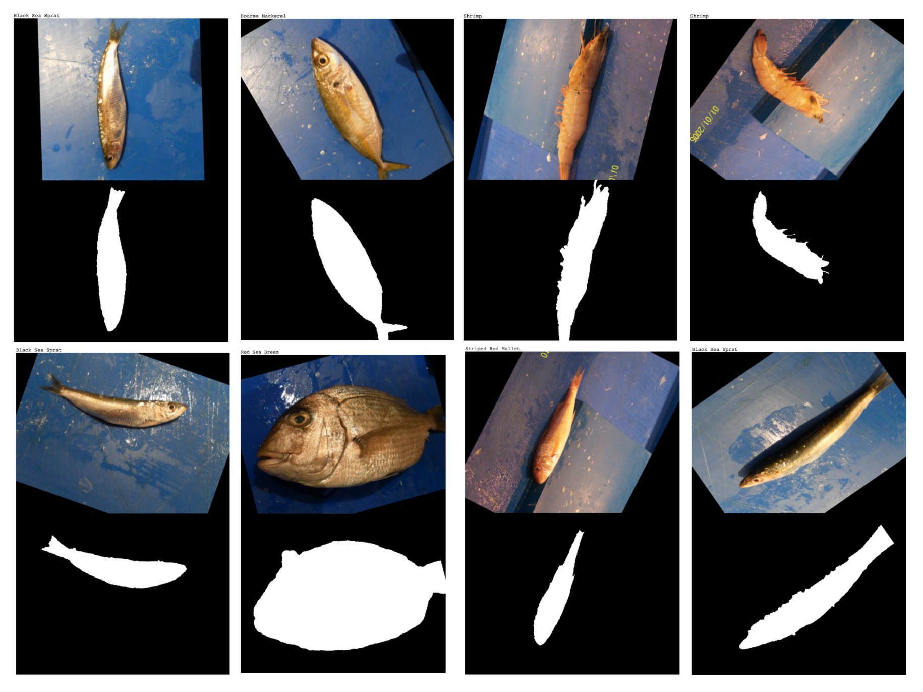
We now have an easy access to the entire organized dataset where each image is stored with its segmentation mask and label! The dataset is available at the public URL: ‘hub://margauxmforsythe/fish_dataset_parallel_computing’.

Here are our final benchmarking’s results on the time taken to upload the full unzipped Fish dataset to the Cloud:

• AWS CLI: 369.0134469759996 seconds

• boto3 — full unzipped dataset: 3768.327020835 seconds

• Hub: 1047.8884124840006 seconds

• Hub with parallel computing: 182.68960309999966 seconds

Uploading the entire dataset to Hub using parallel computing was 2 times faster than AWS CLI and ~20 times faster than boto3!

So now we have a clean, organized, and easy to access dataset in Hub, and it that took only a few seconds to upload 🏁 We are ready to use this dataset to train a classification/segmentation model!

And this is how you can speed up your Machine Learning Workflow at the very first step! ⏱

The notebook for this tutorial is available on Google Colab.